How To Freeze Multiple Cells In Excel 2016
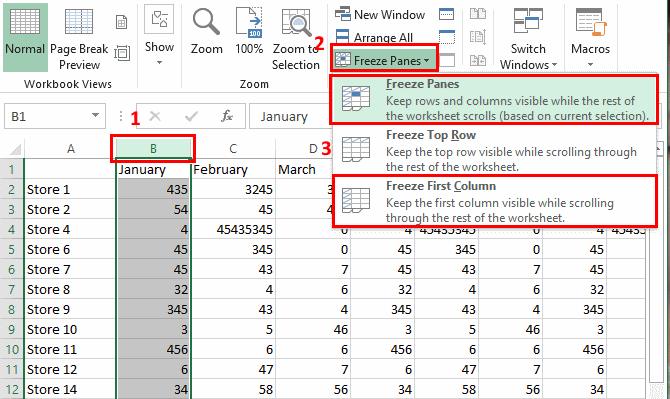
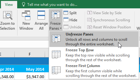
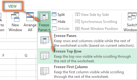
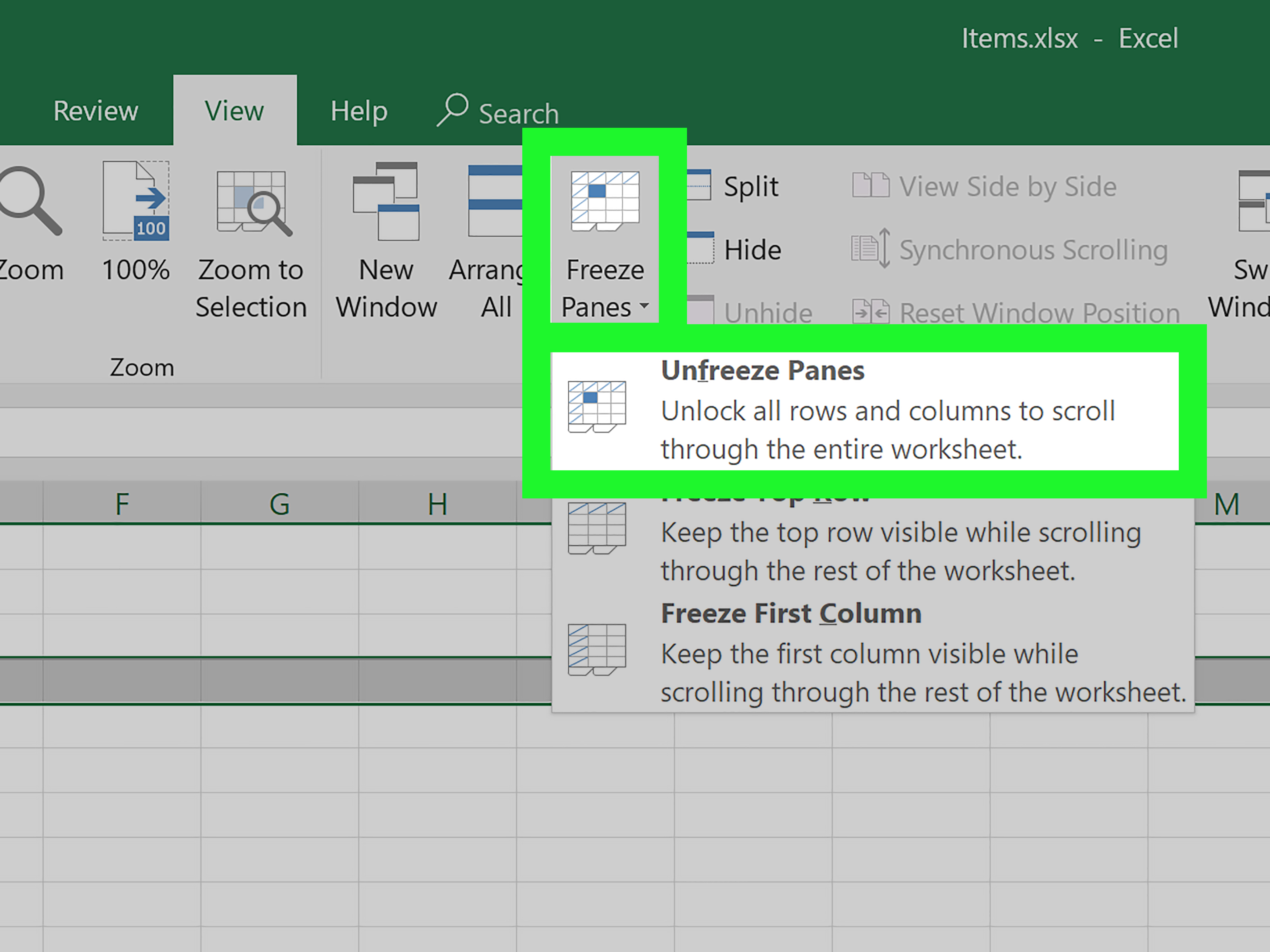
Select View Freeze Panes Freeze Panes. To lock rows select the row below where you want the split to appear To lock columns select the column to the right of where you want the split to appear To lock both rows and columns click the cell below and to the right of where you want the split to appear.
Microsoft Excel Freeze Or Unfreeze Panes Columns And Rows
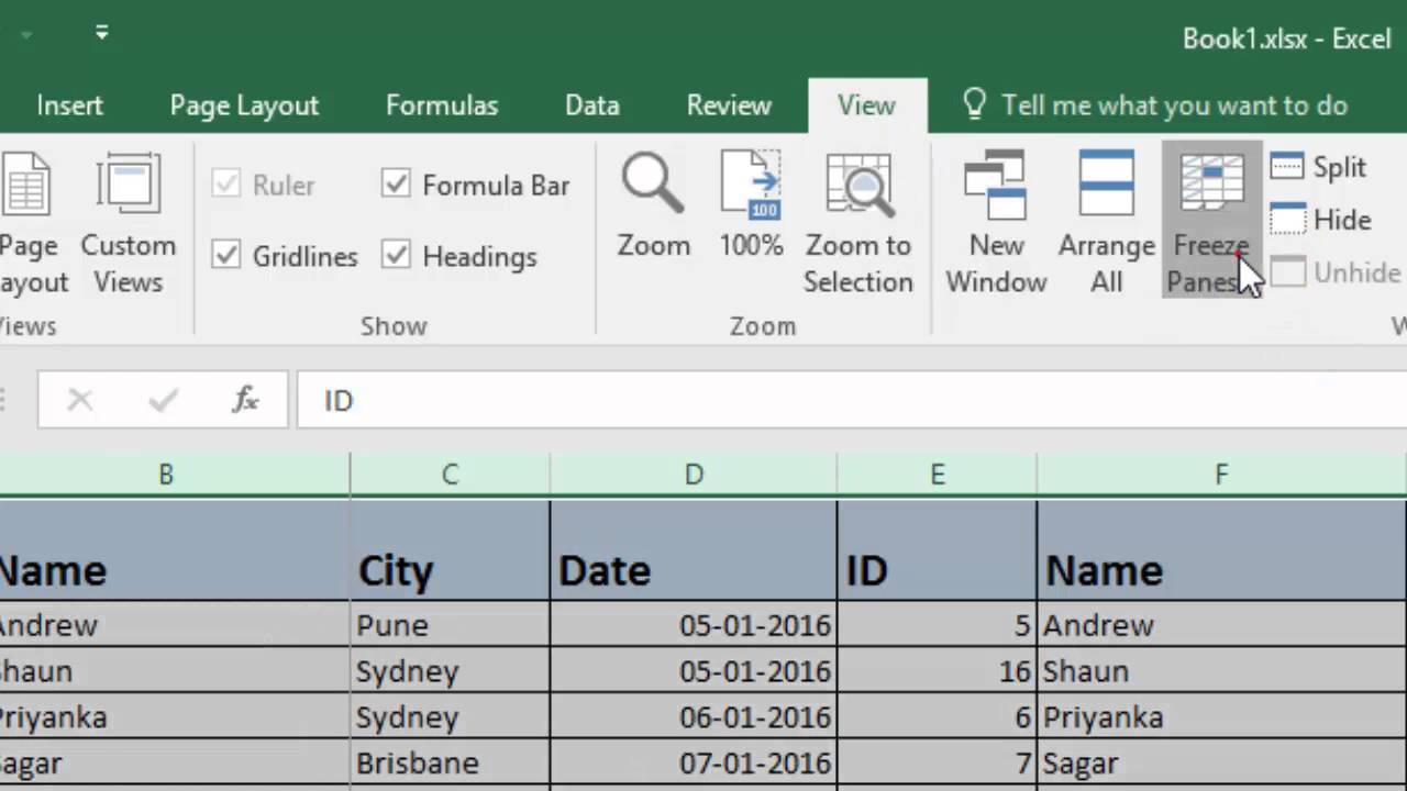
So select either column F or the cell F1.
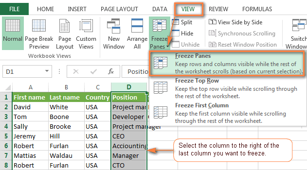
How to freeze multiple cells in excel 2016. How To Freeze Rows In Excel. How To Freeze Multiple Columns In Excel 2016How To Freeze Multiple Columns In Excel 2016 Published at Thursday August 12th 2021 015411 AM by Andrea Rose. Select either the column or the first cell to the right of the last column to be frozen column E.
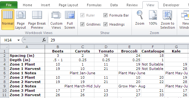
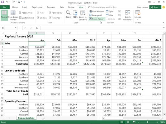
In general its easy to add two data series in one chart in Excel. In this example Excel freezes the top and left pane above row 3 and left of column B. Highlight the data that you would like to use for the line chart.
How to freeze more columns in excel 2016. Open your project in Excel. How to freeze multiple rows in Excel.
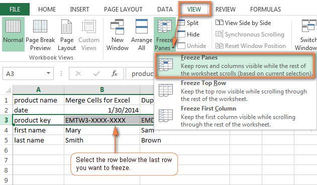
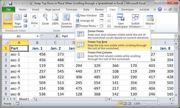
For example to freeze the top row and first column select cell B2 go to the View tab and click Freeze Panes under Freeze Panes. In the Page Setup dialog box click Sheet tab and then select the row or column range that you want to print on each page under the Print titles section see screenshot. The steps to freeze multiple columns in Excel are listed as follows.
The freeze function will allow you to freeze above and or to the left of a selected point on the sheet So the best workaround is to use a helper column. To select place. Insert a new column beside E copy AZ there.
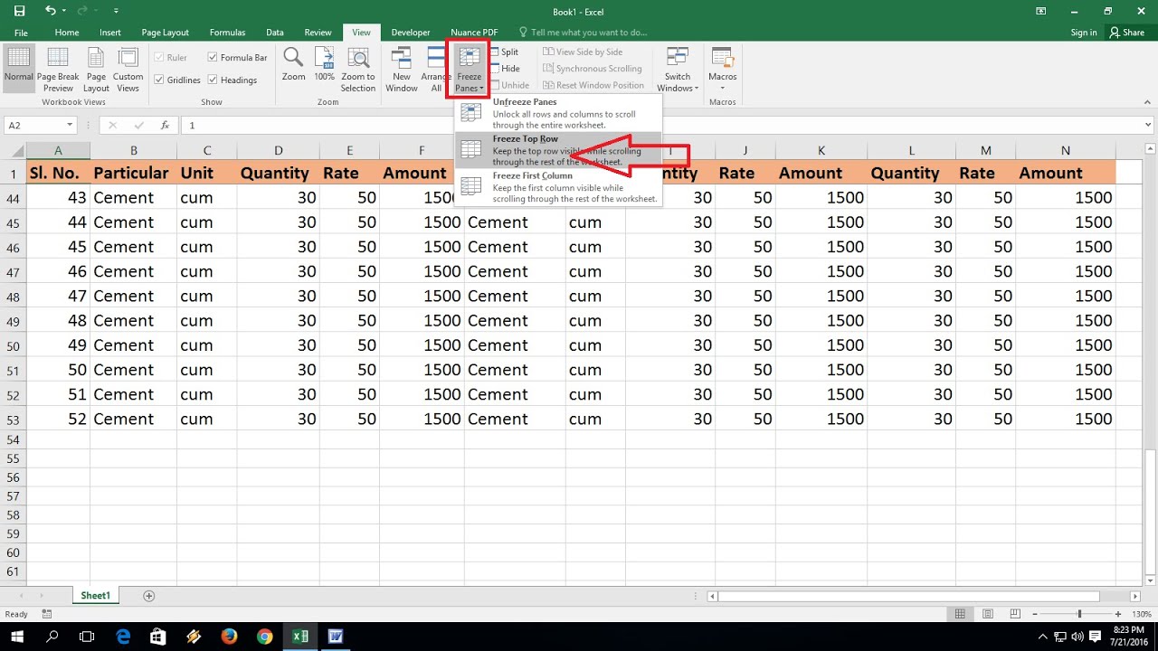
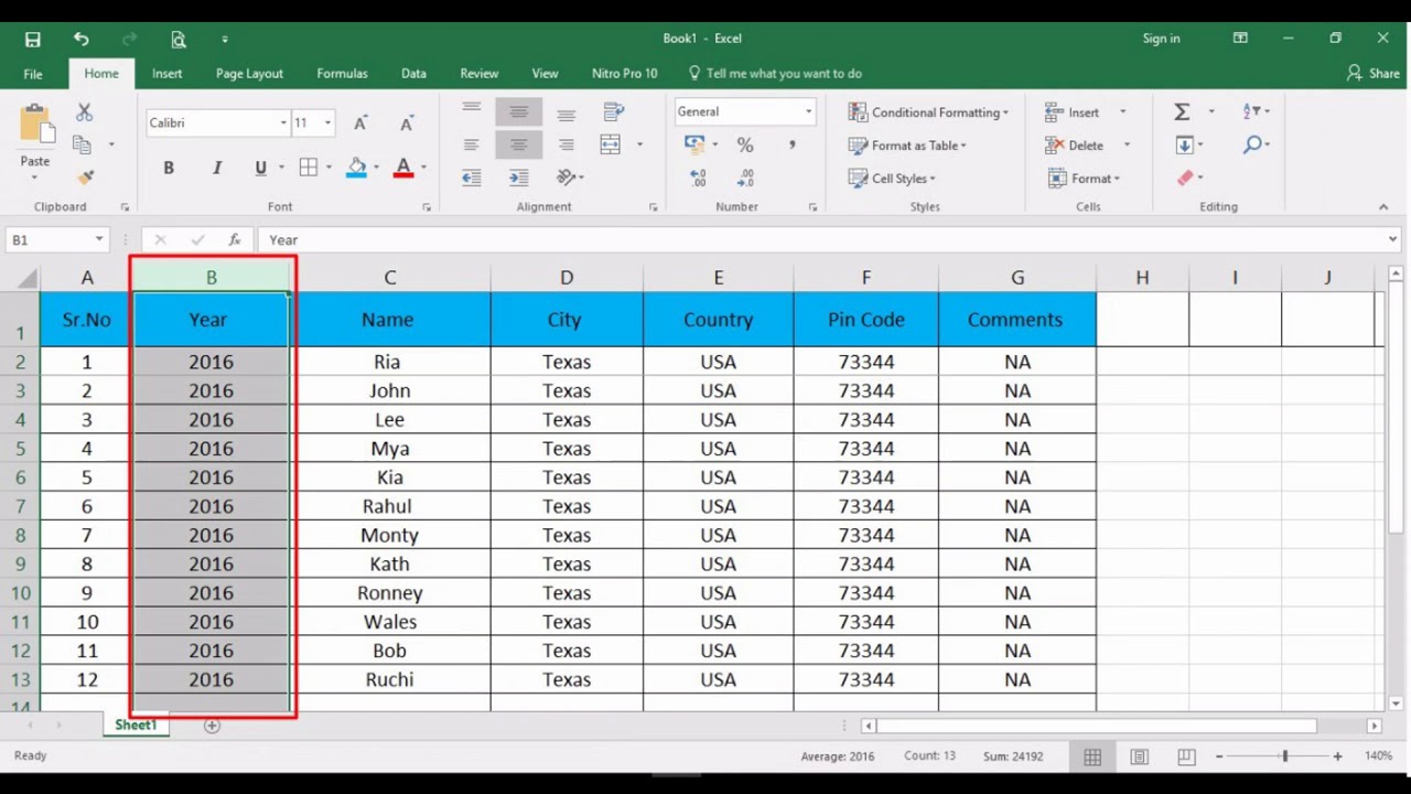
Open the sheet where in you want to freeze the multiple rows and columns keep the first row on top and first column to the left then click next to the cell of the last column and row till where you want to freeze as an example we would like to freeze from Row 1 to 13 and Column A to E so we will click on Cell F14 freeze multiple rows in excel 2016. To create and freeze these panes follow these steps. Steps Download Article 1.
How to freeze top row and multiple columns in excel 2016. The frozen columns will remain visible when you scroll. And then click Print Preview button to view the print result and you can see the frozen header row is always displayed at the top of each.
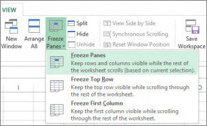
Record some data into an excel sheet if you do not have any existing data records to work on. To do this open Microsoft Excel from your. Click ViewFreeze Panes on the Ribbon and then click Freeze Panes on the drop-down menu or press AltWFF.
This is the step where you highlight or select the rows that you would like to freeze. Now you will see the line Aug 2 2016 Uploaded by TechOnTheNet 14. How do i freeze multiple columns in excel 2016.
Position the cell cursor in cell B3. Freeze rows or columns. Select the Insert tab in the toolbar at the top of the screen.
How may I be able to select more than that first row to freeze. To lock several rows and columns at a time select a cell below the last row and to the right of the last column you want to freeze. You can follow the question or vote as helpful but you cannot reply to this thread.
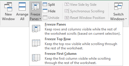
How to Create a Line Chart TechOnTheNet. Freezing more than one row in Excel 2016. In the View tab click the freeze.
About Press Copyright Contact us Creators Advertise Developers Terms Privacy Policy Safety How YouTube works Test new features Press Copyright Contact us Creators. Id like to freeze the first 2 rows in my Excel 2016 spreadsheet but am only able to freeze the top row. How to freeze specific rows and columns in excel 2016.
How to freeze several columns in excel 2016. Open the sheet where in you want to freeze the multiple rows and columns keep the first row on top and first column to the left then click next to the cell of the last column and row till where you want to freeze as an example we would like to freeze from Row 1 to 13 and Column A to E so we will click on Cell. Go the worksheet that you want to print and click Page Layout Page Setup see screenshot.
You can either open the program within Excel by clicking File Open or you can. Youll see this either in the editing. In the same fashion you can freeze as many Excel panes as you want.
How to freeze multiple rows and columns at the same time in excel 2016. Select the cell below the rows and to the right of the columns you want to keep visible when you scroll. This thread is locked.
There is no way of freezing non-continuous columns that Ive seen. Select a cell to the right of the column you want to freeze. How to freeze columns and rows.
I have the same question.
How To Freeze Columns And Rows Microsoft Excel 2016
How To Freeze Multiple Columns In Microsoft Excel Youtube
أكسيل 2016 Freezing Panes اختيارات تجميد الأجزاء لتأمين الصفوف والأعمدة
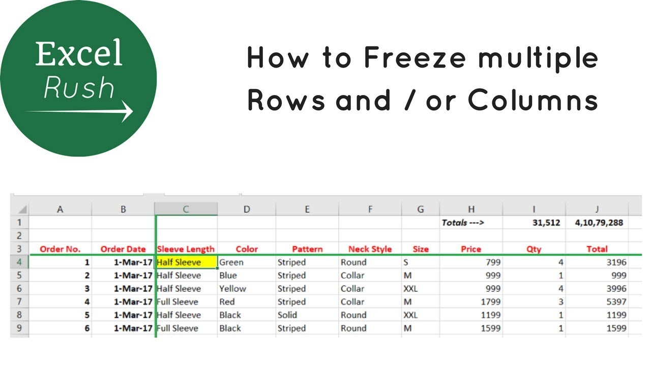
How To Freeze Multiple Rows And Or Columns In Excel Using Freeze Panes Youtube
How To Freeze Panes In Excel Lock Rows And Columns
How To Freeze Panes In Excel Lock Rows And Columns
How To Freeze Panes Rows And Columns In Excel 2016 Youtube
How To Freeze Rows And Columns In Excel

Freeze Panes In Excel
Freeze Or Lock Specific Rows And Columns When Scrolling In Excel Teachexcel Com

Excel Freeze Panes To Lock Rows And Columns
How To Freeze Unfreeze Rows Columns In Ms Excel Excel 2003 2016 Youtube
Excel Freeze Panes To Lock Rows And Columns
Excel How To Freeze Bottom Row And Top Row At The Same Time Youtube
How To Freeze Panes In Excel Lock Rows And Columns
How To Freeze Panes In Excel 2016 Dummies
Excel Freeze Panes To Lock Rows And Columns
How To Freeze Cells In Excel

Simple Ways To Freeze More Than One Column In Excel 5 Steps
Posting Komentar untuk "How To Freeze Multiple Cells In Excel 2016"